
Rebalancing: A fundamental component of investment management
KEY TAKEAWAYS
- Rebalancing is the most efficient and process-oriented way to keep a portfolio on track and is an important part of an advisor’s fiduciary duty.
- Commonly used approaches include buy-and-hold, time-based and drift-based, each of which can have a different effect on maintaining a portfolio’s objective.
- The goal is to determine which rebalancing methodology controls risk on a consistent basis and can be implemented in an efficient and timely manner.
Generally, much time and consideration are put into the client discovery process to determine the most suitable risk/return profile for a client and identify the difference between the ability and the willingness to take risk, so an appropriate strategy is implemented for the client.
An asset allocation strategy is commonly used to control the amount of risk1 to which a client is exposed. Over time, however, if an asset allocation strategy is left to change and drift with the movement of the markets, the risk profile of that strategy will almost surely drift out of line with what was determined to be best-suited for that client.
It is important to maintain the risk and return profile initially determined as appropriate, and establishing a disciplined investment management process is the most effective way to ensure that expectation is met. Typically, more volatile, or risky, asset classes come with higher returns, which potentially leads to those asset classes growing at a faster rate than less volatile asset classes. The inherent risk in these more volatile asset classes increases as the size of the allocation to these asset classes increases. As such, the overall risk of the portfolio can quickly become more than the client is willing or able to bear.
Rebalancing is the practice of bringing the strategy back to the original allocation, and therefore the proper risk profile, by way of selling more volatile asset classes in favor of less volatile ones. Additionally, following an established process can help an investor avoid common mistakes caused by emotional investing. Beach and Rose2 point to three common behavioral finance faults:
- Herd mentality – This is the tendency to do what everyone else is doing. In the case of investing, this means selling assets that are underperforming and buying those that are outperforming. This is counterproductive to overall positive performance of the portfolio.
- Regret aversion – Some investors do not want to admit they’ve purchased an underperforming asset, which leads to holding positions while they continue to lose. This can also include failing to purchase a grossly underpriced asset, even if that is actually the best time to buy it.
- Mental accounting – Some investors also tend to compartmentalize each piece of the portfolio, and fail to understand the benefit of risk reduction through correlation, as well as the importance of how long-term performance contributes to the overall portfolio. This fault commonly leads to herd mentality and regret aversion.
These natural emotional reactions can drastically hinder the success of an asset allocation portfolio and significantly alter the risk/return profile determined appropriate for the investor. As an advisor, there is a responsibility to adhere to the risk expectations outlined in the client’s investment policy statement. Rebalancing is the most efficient and process oriented way in which to keep the portfolio on track and is therefore a very important part of the fiduciary duty an advisor has to his or her clients. This paper addresses a study examining different rebalancing approaches and the effect each had on the risk/return profile of three allocations. The various rebalancing approaches are introduced below and followed by considerations for setting rules around asset class drift. The study’s methodology and results are presented, as well as practical considerations for the application of these results.
REBALANCING APPROACHES
The most commonly used approaches are outlined below. While different approaches may be appropriate for different clients, establishing a rebalancing approach for an investment strategy that is applied across all clients holding that investment strategy yields greater efficiencies for an advisor’s practice. Various approaches can be used to keep portfolio characteristics in line with the stated objective, ranging from doing nothing at all to setting very specific volatility-based tolerance bands around the asset classes in the portfolio. Choosing a rebalancing approach should be made only after careful deliberation of the impact the approach has on maintaining the portfolio’s objective.
BUY AND HOLD: Buy and hold is the simplest approach to implement. Once the assets are invested, no changes are made and the assets are free to move with the markets. The assets with the highest returns, and very likely the highest risk over time, will grow the most. Some investors would argue that a buy-and-hold approach can outperform others because a greater allocation to the higher-returning asset classes means a higher return for the overall portfolio. However, this comes at a cost. It is important to keep in mind that as the proportion to these assets grows, so does the risk inherent in those assets. Over a long enough period of time, a conservative portfolio could end up quite aggressive. One study found that a buy-and-hold approach had 20% more return than a fixed-weight rebalancing approach, but almost twice the volatility.3 This could be difficult to reconcile from a fiduciary standpoint.
CONSTANT MIX OR TIME-BASED: With this approach, asset class weightings are brought back in line with the original allocation at regular intervals, such as monthly, quarterly or annually. The interval can be set to any frequency, however, annual rebalancing is most common. A constant-mix approach tends to be the most efficient in terms of process and risk control, which will be further explained in the section outlining the results of the study. It should be noted that more frequent rebalancing can entail more transaction costs, short-term capital gains, and a potential loss of returns, as rebalancing too frequently does not allow sufficient time for the value of the asset class to meaningfully appreciate.
CONTINGENT OR DRIFT-BASED: A drift-based approach sets a threshold, also known as a trigger or tolerance band, around each of the asset allocations and rebalances the portfolio whenever the threshold is breached. Bands can be relative or absolute. For example, a 10% band may be established around a 40% allocation. Using an absolute band, the allocation would be free to drift up to 50% or down to 30% before a rebalancing event is triggered. Using a relative band, the allocation could drift up to 44% or down to 36% before being rebalanced. The advantage of relative tolerance bands is that they adjust to the allocation of each asset class, large or small. For example, a 15% absolute tolerance band would not be appropriate for an asset class with a 10% allocation, whereas a 15% relative tolerance band would be perfectly reasonable. The size of the tolerance band will impact the frequency and size of trades, which can increase overall costs. To minimize transaction costs, one solution is a partial rebalance rather than a full rebalance back to the original target. In the absolute example above, if the asset with a 40% weight and a 10% absolute band moved beyond 50% of the portfolio, it could be rebalanced back to a weight between 40% and 50% rather than fully back to 40%. This solution minimizes costs while keeping the portfolio properly allocated. However, if the portfolio is rebalanced only partially back to the original target, its risk could be slightly higher than that of the original allocation. In addition to asset class weight, there are other factors to consider when determining the tolerance band size. These factors will be discussed in the next section.
Whether choosing to institute a constant-mix approach, a contingent approach, or a combination of the two, the frequency with which the portfolio will be monitored also needs to be defined. With a constant-mix approach, the portfolio is monitored based on the frequency chosen. So if an annual method is selected, the portfolio only needs to be monitored for drift annually. It is important to note here that trades should be placed in a manner that avoids short-term trading costs.
It is more difficult to determine the most efficient monitoring frequency using a contingent approach. Research suggests daily monitoring is ideal for capturing the most value from market fluctuations, because if the portfolio is not monitored daily, opportunities to capture gains or quickly limit losses may be lost in a volatile market. However, monitoring many portfolios daily can be time consuming and difficult and, consequently, is not the most efficient approach. The choice should be the approach that is most administratively efficient while keeping the portfolio aligned with its initial risk profile.
CONSIDERATIONS FOR SETTING DRIFT RULES
In establishing drift rules, several factors require careful consideration and are heavily dependent upon the chosen approach. Additionally, the costs associated with monitoring and trading should be measured when evaluating various approaches.
ASSET CLASS VOLATILITY
Asset class volatility should be considered when determining tolerance bands. Using the same tolerance band for conservative asset classes and aggressive asset classes produces different results. For example, consider a 10% tolerance band around both investment-grade fixed income and emerging markets equity. Due to the more volatile nature of emerging markets equity, it will breach that band in either direction much more often than investment-grade fixed income, a very conservative asset class whose lower volatility would trigger fewer rebalancing events. For this reason, it may be more efficient to set a wider band around more volatile asset classes, unless it is determined that frequent rebalancing is acceptable for the client.
ASSET CLASS WEIGHTING IN THE PORTFOLIO
Absolute and relative tolerance bands produce differing results depending on the size of the asset class in the portfolio. Absolute tolerance bands require asset classes with small allocations to increase significantly more than asset classes with larger weightings in order to trigger a rebalancing event. For example, a 10% absolute tolerance band on a 5% allocation would not trigger a rebalancing event until that allocation grew to 15%, which is a 200% increase; whereas the same band on a 40% allocation would create a rebalancing event when it reached 50%, merely a 25% increase. Considering the same examples using a relative tolerance band of 10%, rebalancing would be triggered if the upper bands of 5.5% and 44% in the 5% and the 40% allocations, respectively, were breached. These are much more realistic experiences. Relative band methods self-adjust based on the weighting of the asset and are often thought to have an efficiency advantage for this reason. Clearly, the asset class weighting in the portfolio is essential in deciding which type of tolerance band is used.
OTHER CONSIDERATIONS
Tax implications, market conditions, and the objective of the portfolio are also important to consider when rebalancing, although this is not an exhaustive list. Tax implications are a major concern and should be given much thought when choosing an approach and asset allocation. Frequent trading and capital gains can generate significant costs in a taxable portfolio, whereas these factors may be less of a concern in a non-taxable portfolio.
Current market conditions can influence the behavior of a portfolio, making certain approaches more appropriate than others at different times. In a study done by Buetow, Sellers, Trotter, Hunt, and Whipple,4 correlation was shown to be a meaningful factor in a rebalancing approach. In a market environment where correlations are very high, the need for rebalancing may be minimal as asset classes will tend to move together, better maintaining the target profile. When correlations are very low, asset classes may drift apart at a faster pace and need more frequent rebalancing. Wider tolerance bands in a positively trending market will allow the asset classes to capture more gains before a rebalancing event occurs. In volatile markets, tighter tolerance bands would trigger frequent rebalancing events, whereas wider tolerance bands would allow more movement before triggering a rebalance. While the benefit of wider tolerance bands is greater opportunity for growth in a positively trending market, there is also greater potential for loss in a downward trending market.
The objective of the portfolio is also an important factor. A more aggressive portfolio can ideally withstand more aggressive rebalancing, such as wider tolerance bands, less frequent rebalancing, or even a buy-and-hold approach, whereas a portfolio with a more conservative objective would need to be monitored more often for drift outside the acceptable allocation.
After a rebalancing approach has been determined based on the portfolio’s objective, clients can then be assigned to the most suitable portfolio based on willingness and ability to bear risk.
While these are the primary considerations when choosing a rebalancing approach, client needs and circumstances may present other concerns to be addressed. Again, there is no one correct approach for all clients, all portfolios, or even all market conditions. The circumstances should be considered as a whole in order to determine what is most appropriate. The following section discusses an empirical study in which the aforementioned approaches were applied to three allocations to assess the impact of each approach over various timeframes.
AN EMPIRICAL CASE STUDY
This paper, addressing a study of rebalancing approaches, used three allocations to equity and fixed asset classes – 50/50, 60/40 and 70/30 – over a 30-year period from January 1, 1986, through December 31, 2015. Additionally, within this 30-year period, 10- and 20-year timeframes were examined to determine whether different market environments impacted the results of the rebalancing approaches.The 10–year timeframe was January 1, 2006, through December 31, 2015, and 20 years was January 1, 1996, through December 31, 2015. The portfolio values at the start of the 10- and 20-year timeframes were the result of the prior years’ market performance and the rebalancing approach applied and, therefore, it is difficult to isolate the market effect from the rebalancing effect on the ending portfolio value. As such, a follow-up study will reset the portfolios to the 50/50, 60/40 and 70/30 values at the historical 10- and 20-year marks to more clearly ascertain the impact of different market environments.
Fixed income was represented by the Bloomberg Barclays U.S. Aggregate Bond TR USD, and the S&P 500 TR USD represented equities.5 Monthly returns as reported by Morningstar Direct were used for all rebalancing approaches and both indices. Ten rebalancing approaches were studied – four constant-mix, or time-based, and six contingent, or threshold. Each rebalancing approach was applied to the nine different scenarios described above, i.e., each allocation for the three time periods. As stated earlier, research suggests daily monitoring is ideal, however monthly monitoring was used due to a lack of data. The results were not surprising, but rather confirmed what was already assumed: an annual rebalancing method best protects the risk profile intended in the original allocation.
CONSTANT MIX: TIME-BASED METHODS
The time-based methods studied were buy-and-hold, annual, quarterly, and monthly rebalancing. With the exception of buyand-hold, all allocations were rebalanced at those intervals regardless of the deviation from target.
Not surprisingly, buy-and-hold had the highest standard deviation, generally by about 200bps, of all methods over all time periods regardless of the allocation, and offered the highest return in three of the nine scenarios. As previously discussed, it is not a surprise that buy-and-hold would result in the highest standard deviation because the equity portion of the portfolio, typically the riskiest, is allowed to grow unconstrained.
Monthly rebalancing provided lower returns than both annual and quarterly rebalancing in all nine scenarios. The more frequently a portfolio is rebalanced, the less opportunity there is to benefit from increasing returns. Returns can be further hindered by high trading costs and possible short-term gain penalties. When a rebalancing event results in adding to an asset class that is underperforming, i.e., it has breached its lower limit, increasing the frequency could result in extended losses if the asset class continues to underperform. On the other hand, the notion of reversion to the mean6 suggests that adding to an underperforming asset class could have a positive result, as the asset value increases and returns compound.
Annual rebalancing was the clear winner of the time-based methods, offering the highest return in seven of nine scenarios, and the lowest standard deviation six of nine scenarios. In those scenarios where annual rebalancing did not have the highest return or lowest standard deviation, it missed the highest return by just a few basis points with significantly less volatility. For example, a 50/50 portfolio over 30 years rebalanced annually returned 8.95% versus 8.98% on a buy-and-hold portfolio, but with a standard deviation of 8.12% versus 9.93%, a notable difference.
FIGURE 1
Figure 1 illustrates a 60/40 portfolio over 10 years. In this case, annual rebalancing not only has the highest return but also the lowest standard deviation, while the buy-and-hold method yielded the highest standard deviation.7 Monthly rebalancing again offered the lowest return

FIGURE 2
Figure 2 illustrates a slightly riskier portfolio, 70/30, over 20 years. Similar results were found with annual rebalancing outperforming the other methods in both return and standard deviation, and buy-and-hold resulting in the highest risk of the remaining methods.
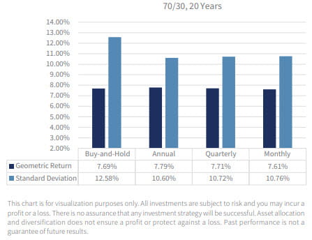
These results support the notion that a buy-and-hold approach is much more risky than other time-based methods and that annual rebalancing offers the best risk control while still providing attractive returns. It could be argued that annual rebalancing may potentially hamper returns when positively trending assets are trimmed back to target, however this was not the case in the present study. As such, when establishing a disciplined investment management process to ensure the portfolio adheres to the risk profile agreed upon with the client, annual rebalancing offers the surest way to achieve that.
CONTINGENT: DRIFT-BASED METHODS
In this study, absolute and relative tolerance bands set at 10% and 20% were examined. Additionally, full and partial rebalancing were studied for the absolute methods. The differences between absolute and relative tolerance bands were described earlier, as well as factors that determine the use of one over the other. Using full rebalancing, the asset class would be rebalanced back to target every time it drifted outside the band, whereas with partial rebalancing, the asset class would be rebalanced back to a predetermined allocation somewhere between the target and the limit of the band. In this study, partial rebalancing back to 50% within the band was used. Based on that, if an asset class with a 20% allocation and a 10% absolute band drifted above 30%, it would be rebalanced back to 25% rather than 20%. The logic behind this is the belief that partial rebalancing can lower trading costs while still allowing the asset room to grow.
As previously mentioned, the sizes of absolute and relative bands produce different results, so deciding which to use and at what size necessitates thoughtful deliberation. Furthermore, the choice between partial and full rebalancing has different implications on the portfolio, in that partial rebalancing can result in more frequent events as the amount of drift required to trigger the event becomes much smaller than intended.
Figure 3
Figure 3 illustrates the difference in drift required in order to trigger a rebalancing event using a relative band versus an absolute band.
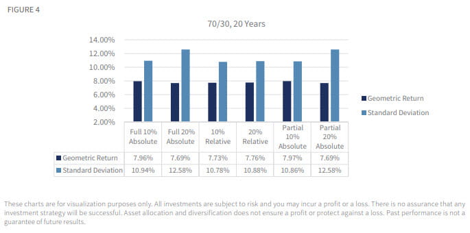
The relative band method did not consistently produce higher returns or lower standard deviations compared to other drift-based methods. In part, this could be due to the higher frequency of rebalancing events triggered when using relative bands. On the other hand, absolute bands produced interesting results. Over a 20-year period, a 70/30 allocation with a 20% absolute band performed most like buy-and-hold because no rebalancing events were triggered from 1996 through 2015. This is why, in figure 4, partial and full 20% absolute show the same return and standard deviation. In fact, the partial 20% absolute method had the highest standard deviation in seven of nine scenarios, in some cases by almost 200 basis points, which is also seen in figure 4 below. Yet, if full rebalancing was used with the same 20% absolute method, it resulted in the highest standard deviation in less than half the scenarios, only four of nine. Perhaps as important, full rebalancing also had the highest return in three of nine scenarios, more than all other drift-based methods except 10% absolute with which it tied.
Using a wider tolerance band on a higher equity-weighted portfolio contributed to these results. And, risk was controlled more consistently when full rebalancing was applied versus only partial rebalancing. Partial rebalancing allowed the equity allocation to remain higher throughout the life of the portfolio and, as such, resulted in greater volatility.
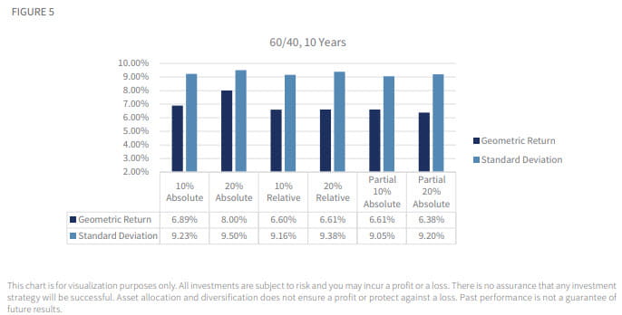
Now consider a very common scenario: a 60/40 portfolio over the 10-year period from 2006 through 2015, illustrated in Figure 5. This is one of the scenarios mentioned above where the full 20% absolute method provided the highest return and highest standard deviation, at 8% and 9.50%, respectively. One rebalancing event occurred when the equity band breached the lower end in February 2009. In this same scenario, the partial 20% absolute method provided the lowest return at 6.38%, with 9.20% standard deviation, and no rebalancing events occurred. Contrary to the 70/30, 20-year example, in a 60/40 allocation over this decade, the two methods behave very differently from one another. Several factors produced this result.
Isolating this 10-year timeframe, which includes 2008, illustrates how a smaller allocation to equities better protected in heavy downturns. However, the impact of partial rebalancing and market conditions over this period also play an important role. At the end of 2005, going into the decade examined here, the equity allocation was 53.52% in the full method versus 64.17% in the partial method. This disparity was due to a rebalancing event in January 1999, where the portfolio was rebalanced to 60/40 in the full method and 70/30 in the partial.
Going into March 2009, after a 37% decline in equities through 2008, the equity allocation of the 60/40 portfolio had declined to 38.47% in the full method, and 49.30% in the partial method. This is where the key difference in performance lies. When the full rebalancing method breached the band at 38.47%, the portfolio was rebalanced back to 60/40 very early in a year where equities then returned 26.46%. By contrast, the band was not breached in the partial rebalancing method, so the portfolio was not rebalanced. As a result, considerably less was allocated to equities and, as such, the portfolio did not benefit as sizably from the correction as the portfolio that experienced full rebalancing.
Over the 10-year period of January 2006 through December 2015, the market performed quite well, and the equity allocation in the full method got as high as 78.56% versus only 70.38% in the partial method.
These nuances, driven by market conditions, led to the outperformance of the full rebalancing method.
CONCLUSION
In this paper, the impact of various constant-mix and contingent rebalancing approaches to the returns and standard deviations of three equity/fixed allocations were examined over three different time periods. As importantly, the paper calls attention to factors that should be incorporated into the decision-making process of choosing a rebalancing approach given the potential impact to the resulting return and standard deviation of the portfolio. Some factors can be planned for, such as trading costs and capital gains, but others, like market conditions, cannot. Regardless, maintaining the portfolio risk profile selected by the client remains the objective for rebalancing. The goal then is to determine which rebalancing methodology controls risk on a consistent basis and can be implemented in an efficient and timely manner. As illustrated in this preliminary study, annual rebalancing does just that.
Across all rebalancing methods, allocations and timeframes, annual rebalancing best controlled risk by providing the lowest standard deviation six of nine times and the highest return seven of nine times.
And, while the results favored a constant-mix approach, the study produced valuable lessons regarding the contingent, or drift-based, approach. Specifically, the use of absolute bands and full rebalancing yielded more favorable outcomes. When absolute bands were used, it resulted in more scenarios where the portfolios had higher returns and/or less risk than when relative bands were used. Full rebalancing back to the original target allocation weight controlled the portfolio’s risk more consistently over various scenarios than only partially rebalancing back within the tolerance band. This study also illustrated that the volatility of and the size of allocation to the asset class moderated the impact to portfolio risk and suggest the use of wider bands when a portfolio is weighted more heavily to volatile asset classes.
Future studies will expand several facets of this initial study. Additional asset classes will be incorporated into the portfolios, as well as different asset allocation blends than those presented here. Specific time periods will be examined. As stated earlier, ten and 20-year time periods did not have the same starting values in this study, which made drawing definitive conclusions challenging. The size of the tolerance bands used will also be varied, perhaps introducing 5% or 15% bands as well. In an effort to determine how robust these initial findings are, it is imperative to take a more critical view into the potential factors impacting portfolio performance and risk.
TERMS/DEFINITIONS
Risk is defined as the chance an outcome or investment’s actual return will differ from the expected outcome or return.
Notion of reversion to the mean is defined as the assumption that prices move toward the average over time.
Standard Deviation measures the variability of the return. A higher standard deviation is indicative of more volatility and a lower standard deviation is representative of lower volatility.
It is important to review the investment objectives, risk tolerance, tax objectives and liquidity needs before choosing an investment style or manager. All investments carry a certain degree of risk and no one particular investment style or manager is suitable for all types of investors.
The content reflects the opinions of Raymond James Asset Management Services and is subject to change at any time without notice. There is no guarantee that these statements or opinions provided herein will prove to be correct. All investments are subject to risk and you may incur a profit or a loss. There is no assurance that any investment strategy will be successful.
1 Risk is the degree to which the returns generated by the asset allocation vary from time period to time period.2 Beach, Steven L. and Clarence C. Rose. “Does Portfolio Rebalancing Help Investors Avoid Common Mistakes?” Journal of Financial Planning, May 2005.
3 Qian, Edward E., To Rebalance or Not to Rebalance: A Statistical Comparison of Terminal Wealth of Fixed-Weight and Buy-and-Hold Portfolios (January 26, 2014). Available at Social Science Research Network (SSRN): http://ssrn.com/abstract=2402679 or http://dx.doi.org/10.2139/ssrn.2402679
4 Overway, C. and Bearce, J. (2010). Rebalancing Multi-Asset Portfolios, Natixis Global Asset Management. http://mpaoverlay.com/cs/ Satellite?c=Document_C&cid=1250208068356&pagename=MPA%2FDocument_C%2FDocument
5 Indices are not available for direct investment. Any investor who attempts to mimic the performance of an index would incur fees and expenses which would reduce returns.
6 Notion of reversion to the mean is defined as the assumption that prices move toward the average over time.
7 Standard Deviation measures the variability of the return. A higher standard deviation is indicative of more volatility and a lower standard deviation is representative of lower volatility.
The foregoing content reflects the opinions of Raymond James Asset Management Services and is subject to change at any time without notice. Content provided herein is for informational purposes only and should not be construed as investment advice or a recommendation regarding the purchase or sale of any security outside of a managed account. There is no guarantee that these statements, opinions or forecasts provided herein will prove to be correct.
All investments are subject to risk and you may incur a profit or a loss. There is no assurance that any investment strategy will be successful. Asset allocation and diversification does not ensure a profit or protect against a loss. Past performance is not a guarantee of future results.
